Knuth’s “Why Pi” Talk at Stanford: Part 1

A few weeks ago I had another opportunity to meet a giant in my field: Donald Knuth was giving his annual Christmas Tree lecture at Stanford, where I happened to be near at the time. The most exciting part was probably right at the very beginning, when Knuth announced that, for the first (“and probably only”) time, he had finished two books on that same day: The Art of Computer Programming: Volume 4A, and Selected Papers on Fun and Games, with the pre-order links on Amazon going up the same day.

The topic of this year’s lecture was, according to the site:

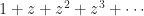
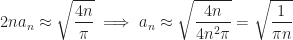
Mathematicians have known for almost 300 years that the value of n! (the product of the first n positive integers) is approximately equal to $\left(\frac{n}{e}\right)^n\sqrt{2\pi n}$ , where $\pi$ is the ratio of the circumference of a circle to its diameter. That’s “Stirling’s approximation.” But it hasn’t been clear why there is any connection whatever between circles and factorials; the appearance of $\pi$ has seemed to be purely coincidental, one of the amazing accidents of nature. Recently however Johan Wästlund has found a nice explanation of this phenomenon, and the reason turns out to be connected with the theory of trees.

I found the lecture originally hard to follow; although Knuth is now 74 years old and physically growing quite frail, his mind was still evidently much sharper than the audience’s; he was completely prepared for every question regarding extensions and corner cases of the material he was presenting. I considered the notes I took to be somewhat useless since I had spent so much time just trying to follow his reasoning. However, when the video became available, I had no excuse left, so I went through it again armed with a pen and the pause button, and I now have a set of notes somewhat worthy of posting here for anyone who missed it. Any errors or inconsistencies are almost definitely my fault and not his.

The notes themselves are after the jump.

There are many combinatorial interpretations of the Catalan numbers, though for the purpose of fitting in with the theme of the lecture, he focused on their correspondence with the number of ordered binary forests on $n$ nodes (although he could just have easily have focused on their more commonly known correspondence with the full binary trees on $n+1$ nodes). Knuth then demonstrated (numerically) the approximation given by

$\displaystyle C_n\approx\frac{4^n}{\sqrt{\pi n}(n+1)}$ ,

and therefore there is some connection between trees and $\pi$ , which he spends most of the talk trying to tease out.

The idea, he says, came from Johan Wästlund‘s article An Elementary Proof of the Wallis Product Formula for pi in the American Mathematical Monthly, Dec. 2007, 914-917. Johan had been searching for ideas for problems for the Swedish Math Olympiad, and came across a problem from Paul Halmos’ Problems for Mathematicians Young and Old. From his description and the snippets from the book’s Amazon page, I’m fairly certain it’s problem 7A on page 53, which reads:

Is it possible to load a pair of dice so that the probability of occurrence of every sum from 2 to 12 shall be the same?

It turns out that this is, in fact, not possible. Knuth says that the proof Halmos gives in this book is complicated and non-elementary (though I can’t check for myself since the Amazon preview sadly doesn’t go that far), but Wästlund wanted to see how a high school student taking the Swedish Math Olympiad might approach it. (It also seems he made the simplifying assumption that the two dice are identical).

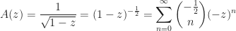
Let $p_i$ be the probability that each weighted die comes up $i$ . Then the probability of 2 coming up when rolling a pair of them can only be $p_1^2$ , which must equal the probability of every other sum, so we obtain

$p_1^2=p_1p_2+p_2p_1\implies p_2=\frac12p_1$

$p_1^2=p_1p_3+p_2p_2+p_3p_1=p_1p_3+\frac{1}{4}p_1^2+p_3p_1\implies p_3=\frac{3}{8}p_1$

$p_1^2=p_1p_4+p_2p_3+p_3p_2+p_4p_1\implies p_4=\frac{15}{48}p_1$ ^[1]

$p_1^2=\ldots\implies p_5=\frac{35}{128}p_1$

$p_1^2=\ldots\implies p_6=\frac{63}{256}p_1$

He noticed an interesting pattern to these coefficients, namely:

$\frac12=\frac12$

$\frac38=\frac12\cdot\frac34$

$\frac{15}{48}=\frac12\cdot\frac34\cdot\frac56$

$\frac{35}{128}=\frac12\cdot\frac34\cdot\frac56\cdot\frac78$

$\frac{63}{256}=\frac12\cdot\frac34\cdot\frac56\cdot\frac78\cdot\frac{9}{10}$

In order to obtain a more general form for these coefficients, let’s say $p_j=a_{j-1}p_1$ . Then consider the generating function $A(z)=a_0+a_1z+a_2z^2+\cdots$ . Squaring it gives us

$A(z)^2=a_0a_0+(a_0a_1+a_1a_0)z+(a_0a_2+a_1a_1+a_2a_0)z^2+\cdots$

However, those coefficients were all chosen to equal $p_1^2=1$ , so that’s really the same as $1+z+z^2+z^3+\cdots$ , which is the infinite series $\frac{1}{1-z}$ . Taking the square root to get back to $A(z)$ , we get

$\displaystyle A(z)=\frac{1}{\sqrt{1-z}}=(1-z)^{-\frac12}=\sum_{n=0}^\infty{\binom{-\frac12}{n}(-z)^n}$ .

Since $A(z)$ was the generating function for $a_n$ , we can conclude that $\displaystyle a_n=\binom{-\frac12}{n}(-1)^n$ . So, for example,

$\displaystyle p_4=\frac{\frac12\cdot\frac32\cdot\frac52\cdot\frac72}{1\cdot2\cdot3\cdot4}=\frac12\cdot\frac34\cdot\frac56\cdot\frac78=\frac{35}{128}$ .

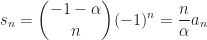
Since we’re talking about probability here, of course we want $p_1+p_2+p_3+p_4+p_5+p_6=1$ , as well as $p_1^2(a_0+a_1+a_2+a_3+a_4+a_5)=1$ . To compute this (and generalizations of this) more easily, we observe that

$A(z)\cdot(1+z+z^2+\cdots)=a_0+(a_0+a_1)z+(a_0+a_1+a_2)z^2+\cdots$

$=s_0+s_1z+s_2z^2+\cdots$

where $s_i=\sum_{k=0}^i{a_i}$ . But since $A(z)=(1-z)^{-\frac12}$ and $(1+z+z^2+\cdots)=(1-z)^{-1}$ , the above generating function is just $(1-z)^{-\frac32}$ so by the binomial theorem again, it equals: $\sum{\binom{-\frac32}{n}(-z)^n}$ . Therefore:

$s_1=a_0=1$

$s_2=a_0+a_1=\frac32$

$s_3=s_2+a_2=\frac32+\frac38=\frac{15}{8}=\frac32\cdot\frac54$

$\vdots$

$s_6=\frac32\cdot\frac54\cdot\frac76\cdot\frac98\cdot\frac{11}{10}$

So it turns out the $s_n$ have just as nice a pattern as the $a_n$ ! In fact, if you plot some rectangles on the plane with borders at each of the $a_k$ (therefore with a total width and height of $s_k$ ), you get a remarkable picture:

Figure 1: Graph for s₁₀. As k grows, the resemblance to a circle becomes even more striking

I think this is the point where most of us began to see where the talk was going; since the big red block in the bottom-left corner represents $p_1^2$ , it has an area of 1, and every other color has to add up to the same sum. Since there’s ten such colors, the total area of this region is 10. However, it’s quite obviously also approximating a quarter-circle of radius $s_{10}$ ! Indeed, if we could prove that the circle will always only intersect the outermost layer of blocks, then we could bound the error of this approximation with

$\displaystyle n-1<\frac\pi4s_n^2<n+1$

So here’s the “cute proof”^[2] that the above holds.

Notice that $\displaystyle\left(1+\frac{1}{2k}\right)^2=1+\frac1k+\frac1{4k^2}>1+\frac1k$ . Similarly,

$\displaystyle\left(1+\frac{1}{2k}\right)^2=1+\frac1k+\frac{1}{4k^2}<1+\frac1k+\frac{1}{k^2}+\frac{1}{k^3}+\cdots$

since $\frac{1}{4k^2}<\frac1{k(k-1)}$ . From the formula, $s_{a+b}^2=s_{a}^2\left(\frac{2a+1}{2a}\right)^2\left(\frac{2a+3}{2(a+1)}\right)^2\cdots\left(\frac{2(a+b-1)+1}{2(a+b-1)}\right)^2$ so by applying the two inequalities from before, we arrive at the important inequality:

$\displaystyle s_a^2\left(\frac{a+b}{a}\right)<s_{a+b}^2<s_{a}^2\left(\frac{a+b-1}{a-1}\right)$

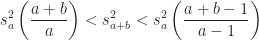
Now, the inner notches of the shape in Figure 1 occur at coordinates $(s_k,s_{n-k})$ which we want to show is inside the circle. That is, we want to show $s_{k}^2+s_{n-k}^2<s_{n}^2$ . Using the formula above we know

$\displaystyle s_k^2\leq s_{n-k}^2\left(\frac{k-1}{n-k-1}\right)\leq s_{n}^2\left(\frac{n-k-1}{n-1}\right)\left(\frac{k-1}{n-k-1}\right)=s_n^2\left(\frac{k-1}{n-1}\right)$ .

So,

$\displaystyle s_k^2+\left(\frac{n-k-1}{k-1}\right)\left(s_{n-k}^2\left(\frac{k-1}{n-k-1}\right)\right)<\left(1+\frac{n-k-1}{k-1}\right)\left(\frac{k-1}{n-1}\right)s_n^2$

$\displaystyle =\left(\frac{k-1+n-k-1}{k-1}\right)\left(\frac{k-1}{n-1}\right)s_n^2$

$\displaystyle =\left(\frac{n-2}{n-1}\right)s_n^2<s_n^2$

A similar trick using the other inequality works for the outer notches as well, so we have justified the earlier bound on $\frac\pi4s_n^2$ in completely elementary terms. This shows how $\pi$ is related to $s_n$ . Now we just have to turn this into factorials. Recall that $a_n=\frac12\cdot\frac34\cdots\frac{2n-1}{2n}$ , and that $s_n=2na_n$ . Since we have just finished proving that $\frac\pi4s_n^2\approx n$ we know that $s_n\approx\sqrt{\frac{4n}\pi}$ , so:

$\displaystyle 2na_n\approx\sqrt{\frac{4n}\pi}\implies a_n\approx\sqrt{\frac{4n}{4n^2\pi}}=\sqrt{\frac1{\pi n}}$

And there we have it: a simple link between factorials and the circle. It turns out that you can play the same game with any other “super-ellipse” of the form

$\displaystyle x^{\frac1\alpha}+y^{\frac1\alpha}=r^{\frac1\alpha}$

of which the circle is only one special case ( $\alpha=\frac12$ ). You just have to choose a different set of coefficients:

$\displaystyle a_n=\binom{-\alpha}{n}(-1)^n$

$\displaystyle s_n=\binom{-1-\alpha}{n}(-1)^n=\frac{n}{\alpha}a_n$

$\displaystyle b_n=a_0a_n+\cdots+a_na_0=\left(\frac{1-\alpha}{n}\right)(-1)^n$

$\displaystyle \text{area}=b_0+\cdots+b_n=\binom{n-\alpha}{n-1}$

Following the same sort of logic (claims Knuth) will allow you to approximate the area of the corresponding super-ellipse, which is

$\displaystyle \frac{2\alpha\Gamma(\alpha)^2}{\Gamma(2\alpha)}$

Notice that $\Gamma(\frac12)=\sqrt\pi$ and $\Gamma(1)=1$ , which shows what we’ve really been approximating all along!

The method apparently even works in three dimensions, just by calculating the coefficients for three dice rather than two. He provided the following image to whet our appetites.

Figure 2: Approximate ball for three die

The rest of the talk focused on another combinatorial interpretation of $a_n$ which has applications to coding theory, and a relatively uninteresting Q&A session that nevertheless did have one gem in it: a problem relating $\pi$ to random mappings which Knuth cannot figure out. I’ll write in detail about both of these things in future blog posts, though, because this one has already become prohibitively large. I hope someone finds it interesting 🙂

[1]: Actually, he consistently wrote $\frac{15}{16}$ throughout the whole talk, but the correct value is really $\frac{15}{48}$ .
[2]: His words, not mine!

Written by Adrian Petrescu

December 28, 2010 at 4:41 am

Posted in Computer Science, Mathematics

Tagged with Knuth, Math

6 Responses

Subscribe to comments with RSS.

awesome! thanks! I wasn’t there, but I am surprised that nobody nitpicked the 16/48 mistake 🙂

Alessandro

January 2, 2011 at 7:19 pm

Reply
- Yeah, I wonder if I had pointed it out if it would’ve gotten me one of those six free books 🙂
  
  Adrian Petrescu
  
  January 2, 2011 at 7:31 pm
  
  Reply
Buna – vroiam sa iti spun ca, in calitatea unui adolescent care spera sa studieze comp sci in viitor, te admir si iti urez succes in proiectele tale 🙂

vladh

May 5, 2011 at 5:03 pm

Reply
Why is it that a 2D random walk is recurrent, while a 3D random walk is transient?…

Very nice answer, Alon! One quick note about the ‘naturalness’ of [math]\sqrt{n}[/math] in Stirling’s Approximation. There is a paper by Feller (“A Direct Proof of Stirling’s Formula”, Am. Math. Monthly, 1967) that gives us some intuition for th…

Quora

October 21, 2012 at 7:06 pm

Reply
[…] Stirling’s Approximation […]

Metric Learning: Some Quantum Statistical Mechanics | Machine Learning

November 14, 2013 at 5:03 pm

Reply
Adrian, You have done an excellent job. Since you have transcripted both part 1 and part 2 of Prof Knuth’s lectures, with mistakes corrected, how about getting all his mathematical lectures (in case you have done this to his other math videos as well) published in a book form with his permission? A great opportunity of doing something with such an eminent person.

C.Rama Murthy

January 30, 2015 at 4:06 am

Reply